
Machine Learning
Linear Algebra in Machine Learning
Learn vectors, matrices, dot products, and eigenvalues through simple explanations and real-world examples.
In my first blog, Understanding Mathematics in Machine Learning : Math Made Simple, I had simplified the Mathematics in Machine Learning. Now, let's go a level deeper with all those concepts, starting with Linear Algebra.
Machine Learning models do three main things:
1. Represent data
2. Transform data
3. Extract patterns
All these are done using vectors and matrices.
When you create a model and run this command:
model.fit(X, y)
Have you ever wondered what happens behind the scenes?
You’re actually triggering thousands (sometimes millions) of matrix operations.
What is a Vector in Machine learning?
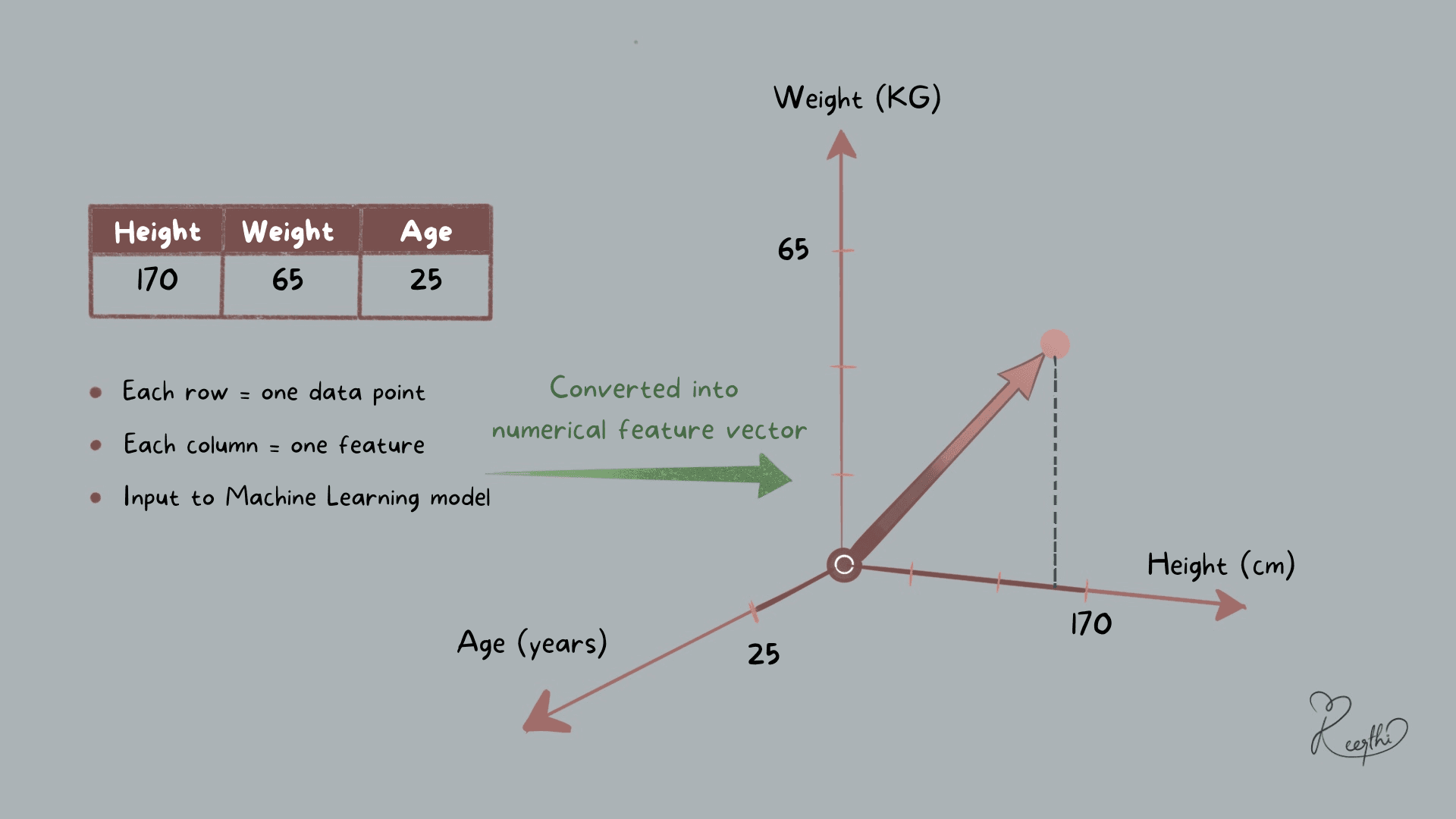
At its simplest, a vector is just a list of numbers.
Example:
A person in a dataset:
Height = 170
Weight = 65
Age = 25
We represent this as:
x=[170,65,25]
This is called a feature vector. Every data point in your dataset is a vector.
If you have 1000 rows in your dataset → You have 1000 vectors.
1. What Does “Vector as an Arrow” Really Mean?
In mathematics, a vector like:
v=[3,4]
means,
Move 3 units in the x-direction and Move 4 units in the y-direction
This forms an arrow from the origin to the point (3,4).
Magnitude (Length)
The length of the arrow. For [3,4], the magnitude is:
It tells us how large the vector is.
Direction
The angle at which the arrow points.
It tells us which way the vector is oriented.
2. Dot Product — The Core Operation in ML
Suppose,
The dot product is:
This is exactly what happens in:
Linear Regression
Logistic Regression
Neural Networks
When we compute:
That’s a dot product. Dot product answers this question:
How aligned are these two vectors?
If they point in similar directions → high value
If they are unrelated → small value
If opposite → negative value
In NLP, cosine similarity (used in embeddings and search engines) is based on dot product.
So yes — even modern AI systems rely on this simple operation.
3. What is a Matrix?
If a vector represents one data point, a matrix represents the entire dataset.
Example:
Rows → samples
Columns → features
Every dataset in Machine Learning is stored as a matrix.
When you load data using pandas or NumPy, you are working with matrices.
4. Matrix Multiplication
Neural networks follow a simple rule:
Output=XW+b
Where,
X → input matrix
W → weight matrix
b → bias
That’s it.
Deep learning is repeated matrix multiplication followed by activation functions.
Even CNNs and Transformers are optimized matrix machines.
At this point, it’s easy to confuse the Dot Product you read earlier and with the Matix Multiplication— but they are not the same thing.
Dot Product
Happens between two vectors and produces a single number (scalar)
Example:
[1,2,3] ⋅ [4,5,6]= 1×4 + 2×5 + 3×6 = 32
Output is just one number.
Matrix Multiplication
Happens between matrices (or matrix and vector) and produces another matrix (or vector)
Example:
Output is a vector, not a single number.
5. Eigenvalues & Eigenvectors — Finding Important Directions
Now this sounds complex, but here’s the intuition. Imagine your data points are scattered in 2D space. Some directions show more variation than others.
In mathematical terms:
A v = λ v
Here,
A is a matrix representing the transformation,
v is the eigenvector,
λ is the eigenvalue.
“Applying the transformation A to the vector v just stretches it by λ, without changing its direction.”
Eigenvectors tell us:
The direction where variance is maximum means the direction where your data spreads the most
Eigenvalues tell us:
How important that direction is.
Large eigenvalue → very important direction
Small eigenvalue → less useful direction
Real World Applications in ML:
PCA (Principal Component Analysis)
Dimensionality Reduction
Noise removal
Principal Component Analysis (PCA): Reducing the dimensions of huge datasets by finding the directions (principal components) with the most variance.


